Exoplanet Transits: How Our Predictions Stack Up

Compare the system parameters derived on the worksheet from the canonical values you can find online in Exoplanets.org.

Before we start, let's just take a moment to consider the fact that there's a website (actually there are several such websites) where you can look at the data on hundreds upon hundreds of exoplanets, from their mass to their radius to the properties of their orbit and parent star.

If that doesn't just blow your mind, I don't know what will.

With that out of the way, let's look at the quantities we estimated two posts ago, and how they stack up against the values found here.

Size comparison of Jupiter (L) and WASP 10b (R) (source).

We estimated $R_p$ to be 1.3 Jupiter radii; Exoplanets.org has it at 1.08 Jupiter radii (16% error).

We estimated $M_*$ to be 0.790$M_\odot$; Exoplanets.org has it at 0.790$M_\odot$ as well(!) (0% error).

We estimated $M_p$ to be 5.27 Jupiter masses; Exoplanets.org has it as 3.19 Jupiter masses (39% error).

We estimated $a/R_*$ to be 12; Exoplanets.org has it as 11.87 (0.3% error).

We estimated $T$ to be 2 hours ($7.2 \times 10^3$ seconds); Exoplanets.org has it at $8.0 \times 10^3$ seconds) (10% error).

We estimated $\rho_*$ to be 3.4 g cm$^{-3}$; Exoplanets.org has it at 1.5 g cm$^{-3}$ (130% error).

We estimated $\rho_p$ to be 2.8 g cm$^{-3}$; Exoplanets.org has it at 3.1 g cm$^{-3}$ (9% error).

These are all pretty impressively close, with a couple of exceptions (most notably the stellar density). However, even those discrepancies don't look too bad when you consider that we were working with a given stellar radius of $0.8M_\odot$--the canonical value is actually just short of $0.7 M_\odot$, which would notably improve a our value for stellar density.

All in all, a pretty impressive show for just a couple of graphs and some algebra!

Survivable, More or Less: Stellar Habitable Zones

Now let's figure out what stars make the best targets for both the radial velocity technique and the transit method, assuming we are primarily interested in finding planets in their stars' habitable zones. For a planet in the habitable zone of a star of mass $M_*$...

The habitable zone is a pretty simple, and neat, idea--essentially, for a given star of a given size (and temperature, and luminosity--but, as we know, these parameters are all connected), there is a range of radii out from the star called the habitable zone which is just the right temperature for liquid water to exist on a planet's surface (for this reason it's also known as the "Goldilocks zone"--not too hot, not too cold).

Habitable zones as a function of $M_*$ (source).

Unfortunately, this is one of those ideas that sounds a lot better than it works. In reality, there are a ton of different factors that could influence where planets (or moons!) could be habitable, from atmospheric composition (imagine a planet as far from the Sun as Mars but with Venus' wicked greenhouse atmosphere), internal heating due to tidal forces (looking at you, Europa), and reflected sunlight from a large parent planet in the case of moons. This is all assuming that liquid water is a must for life, which is a big if. However, despite the oversimplifications inherent, it's still an interesting concept to explore.

a) How does the Doppler amplitude, $K_{HZ}$, scale with stellar mass?

Doppler amplitude is a scary sounding term, but it's actually something we've gotten pretty familiar with at this point--the maximum radial velocity of the star, $v_*$. As we know, $M_p v_p = M_* v_*$. We can treat $M_p$ as a constant, so if we divide $M_*$ over to the other side, we can turn this into a scaling relation based on mass and velocity:\[v_* - K_{HZ} \sim \frac{v_p}{M_*}\]So our next step is to figure out how $v_p$ scales with stellar mass. Assuming a circular orbit, we know that $v_p = \frac{2\pi a}{P} \sim \frac{a}{P}$, so we can substitute into our scaling relation to get \[K_{HZ} \sim \frac{\frac{a}{P}}{M_*}\]According to Kepler's Third Law, $P \sim (\frac{M_*}{a^3})^{1/3}$, so we can substitute this in as well. \[K_{HZ} \sim a^{-1/2}M_*^{-1/2}\] Bear in mind that this isn't an arbitrary $a$, this is actually $a_{HZ}$--the distance of the habitable zone from the parent star, which scales as $T^{-2} L^{1/2}$. If we hold temperature constant and use the (fuzzy, but reliable) intermediate-mass mass-luminosity relation for main sequence stars $L \sim M$, we can say that $a_{HZ} \sim L^{1/2} \sim M_* ^2$. Plugging this back into our relation for $K_{HZ}$ gives us a final scaling relation:\[K_{HZ} \sim M_* ^ {-\frac{3}{2}}\]
b) How does the transit depth, $\delta$, scale with $M_*$?

In our recent examination of exoplanets we found that $\delta \sim \frac{R_p ^2}{R_* ^2}$. We're holding $R_p$ constant, so all we're interested in is how $M_*$ scales with $R_*$. This is actually a hotly investigated question for parts of the H-R diagram (particularly low-mass stars), but in the region close to one solar mass (where most stars are located), it's pretty reliably $M \sim R$. Thus, we can simply substitute radius for mass into our scaling relation to find that \[\delta \sim M_* ^{-2}\]
c) How does the transit probability, Prob$_{tr, HZ}$, depend on $M_*$?

The transit probability is exactly what it sounds like--the likelihood that an observable transit of an exoplanet (in this case in the habitable zone) will occur. Transit probability is equal to $\frac{R_*}{a_{HZ}}$, so this is again a simple matter of substituting according to other scaling relations--$R\sim M$ for $R_*$ and $a_{HZ} \sim M^2$ for $a_{HZ}$. The result:\[\textrm{Prob}_{tr,HZ} \sim M_* ^{-1}\]
d) How does the number of transits (orbits) per year depend on stellar mass?

The longer a planet's orbital period is, the fewer transits we'll see in a given year--so, intuitively, the number of transits per year scales as $P^{-1}$. We found in part a) that $P \sim \frac{a_{HZ}^{3/2}}{M_* ^{1/2}} \sim M^{5/2}$, so we then know that\[N_{transits} \sim M^{-5/2}\]
e) Based on this analysis, what are the best kinds of target stars for the search for habitable zone planets? What factors did we ignore in this analysis?

All the results we found scaled inversely with mass--in other words, increasing the mass of a target star decreases the amplitude of Doppler shifts, the transit depth, the likelihood of a transit, and the number of observable transits per year. The obvious conclusion is that we should target the smallest stars we can possibly find. However, our simplifying assumptions eliminated a few factors that can be pretty crucial when searching for exoplanets. We ignored temperature entirely, despite the fact that some stars, such as brown dwarfs (semantic discussion of whether brown dwarfs count as stars notwithstanding) are so cold that it would be absurd to search for habitable planets around them--one, discovered recently, is literally as cold as water ice. Perhaps most importantly, though, we disregarded the brightness of our target stars. Dimmer stars around one solar mass may be the most common stars in the galaxy, but brighter A-types--despite being 0.5% as common--constitute the bulk of easily observable stars, since they can be seen from orders of magnitude farther away. Thus, in conducting a wide-ranging search for exoplanets, it is important to balance the competing factors of mass and visibility.

Credit and appreciation go to Anne Madoff, Scott Zhuge, Jennifer Shi, and Louise Decoppet for collaboration on these problems.

Exoplanet Transits: The Bread and Butter of Detecting Other Worlds

What properties can be obtained from a planetary transit lightcurve and radial velocity curve?

This is a pretty general question, so it's important to start by examining what data we actually collect when we observe the radial velocity of a star and the light curve of a planetary transit. The first of these, the radial velocity curve, we have actually already discussed in great depth here, but we'll do a quick refresher course on that when we get around to using it. Right off the bat, though, we'll be working with the planet's lightcurve.

Lightcurve of WASP-10 b transit.

As you can see, there's a very obviously visible dip in the amount of light we're receiving from the host star, WASP-10, as the planet passes in front of it. As a matter of fact, we can derive a pretty substantial amount of information from the length, depth, and shape of this dip. 

The sharply slanted edges are known as "ingress" and "egress," and are the time it takes for the planet to go from just barely overlapping with the outer edge of the star to sitting entirely in front of it. However, in between ingress and egress the brightness of the star isn't constant--it actually keeps getting dimmer until the very center of the transit. This is due to a process called "limb darkening," where the outer edge of a star's disc actually appears less bright than the center (it has to do with looking through more of the star's atmosphere, and is comparable to why stars are dimmer and harder to observe when they're close to the horizon). This phenomenon is easily visible on any high-resolution image of the Sun:

Example of limb darkening on the Sun (source).

We can also figure out the relative radii of the planet and star from the depth of the transit. Since the planet is emitting essentially no light, the flux received from the star should decrease by a factor equivalent to the area of the planet's disc ($\pi R_p ^2$) over the area of the star's disc ($\pi R_* ^2$), since the planet is blocking that fraction of the star's area, and thus light. If we define the depth of the transit as $\delta$, we can express this mathematically as\[\delta = \frac{R_p ^2 }{R_* ^2}\]On our lightcurve of WASP-10 b it looks like $\delta$ is around 0.3, so we know that the radius of the planet is around $\sqrt{0.03} \approx 1.7 \times 10^{-1}$ times  the star's radius.

The next thing we can figure out from the lightcurve is the ratio of the star's radius to the planet's orbital semimajor axis.

The star on the left, with the planet shown at the start of its transit (top) and end of its transit (bottom). The orbital semimajor axis, a, and the radius of the star, $R_*$, are labeled.

As you can immediately see from the figure above, $tan(\theta) \approx \theta = R_*/a$. The ratio of the transit time to double this angle will be the same as the total period over the angle traversed over one period ($2\pi$, a full circle). Or, in equation form: \[\frac{t_t}{2\theta}=\frac{t_t}{\frac{R_*}{a}}=\frac{P}{2\pi}\]Rearranging this, we can see that the ratio of $a$ to $R_*$ is \[\frac{a}{R_*} = \frac{P}{2\pi t_t}\]If we had a longer lightcurve showing multiple transits we would be able to pull the period off of that, but we can also grab it off of the radial velocity curve (which will make an appearance in a few moments). As it happens, WASP-10 b has a 3.1-day period (meaning the planet's year lasts only 3.1 days!), and from the lightcurve we can tell that the transit time is right around 2 hours, so we can tell that the semimajor axis is 3.1 days/2 hours $\approx$ 12 times the radius of the star.

Now it gets both very messy and very cool. Density is defined as mass over volume, so we know that\[\rho_* = \frac{M_*}{4/3 \pi R_*^3}\]. We can also solve Kepler's third law for $a$ to give us \[a = \left(\frac{GM_*P^2}{4\pi^2}\right)^{1/3}\] The algebra from here gets sloppy and hard-to-follow, so we'll skip to the interesting part (if we were writing a textbook, this is where we would say that "the derivation is left as an exercise"). We can put these equations togetehr and solve for the density of the star in terms of known quantities, including the ratio of the semimajor axis to the star's radius:\[\rho_* = \left(\frac{a}{R_*}\right)^3\left(\frac{3\pi}{GP^2}\right)\]In the case of WASP-10, this gives us a density of 3.4 g cm$^{-3}$, or about 2.4 times the density of the Sun.

If we know the radius of the star, we can now figure out a few more definite quantities. Let's say $R_* \approx 0.8R_\odot$. From our semimajor axis-radius ratio, we can immediately say that WASP-10 b is orbiting at $12 \times 0.8 R_\odot = 6.7 \times 10^11$ cm. Since we also have an equation for the ratio of the planetary and stellar radius, we can also say that $R_p = 0.17 \times 0.8 R_\odot = 9.5 \times 10^9$ cm. Since we know the density of WASP-10, we can also compute its mass as $M_* = 3.4 \times 4/3 \pi (0.8 M_\odot)^3 = 2.5 \times 10^{33}$ g, or 1.2 $M_\odot$. The last value we can compute is the radial velocity of the planet, $K_p$. If we assume a circular orbit (and thus constant velocity), this means that $K_p$ can be related to $P$ and $a$ in a distance-rate-time equation, $K_p \times P = 2\pi a$. Solving for $K_p$ gives us a brisk $1.5 \times 10^7$ cm s$^{-1}$.

To continue, we'll finally break out that radial velocity chart.

As you can see, the star's radial velocity fluctuates from around -500 m/s to 500 m/s. This means that it's actually steadily moving around its orbit at this speed--we just only see it moving at that speed when it's going directly toward or away from us (remember, it's a radial velocity plot). Back when we were looking at these earlier, we found that $M_* v_* = M_p v_p$. Luckily for us, we've figured out three out of these four variables, and can now solve for the mass of the planet using the mass of the star and the radial velocities of each--it comes out to $M_p = 10^{31}$ g.

Lastly, but still important, we can figure out a quantity called the "impact parameter," which we'll denote as $b$. This is a value between 0 and 1 which quantifies how close the planet is to transiting directly across the star's equator ($b = 0$) and just skirting its edge ($b=1$).

Visualization of the impact parameter $b$. The planet moves along the horizontal line at the top (source).

$b$ is related to the depth of the transit $\delta$, along with the total transit time $T$ and the ingress time $\tau$ according to $b = 1 - \delta^{1/2}\frac{T}{\tau}$. We can estimate $\tau$ from the light curve to be about 0.3 hours, so finding $b$ is a simple matter of plugging and chugging--it comes out to be about 0.13.

So, summing everything up--from two plots and a given radius, we were able to find:

-The length of an exoplanet's year
-The density of its host star
-The mass of its host star
-The mass of the exoplanet itself
-The radius of the exoplanet
-The radial velocity of the exoplanet
-The radial velocity of the star
-The impact parameter of the planet.

We didn't do this, but we can also find the density of the exoplanet--it's an easy matter of dividing mass by volume. As it turns out, in this case $\rho_p = 2.8$ g s$^{-1}$.

Lots of thanks and credit goes to Anne Madoff, Scott Zhuge, Jennifer Shi, and Louise Decoppet for helping out with this one.

HR 8799 and the Vortex Coronagraph

(source)

This is a pretty cool picture--one that I think really is worth its own post. It's a direct image of the three planets known to orbit the star HR 8799. HR 8799 is an exceptionally young star--just 30 million years old or so--and it is still surrounded by an enormous dust halo over 2000 AU in diameter. This cloud of dust is apparently so thick that it threatens the stability of this young solar system. and could be the subject of a post all its own. However, it is not the subject of this post. The three planets known to orbit inside of it are (actually, there are four--but one is too close in to directly image yet) .

Those three imageable planets were among the first directly imaged, using the Keck telescopes in 2008, observed using adaptive optics in infrared. But the image we're concerned with here is an entirely different image, taken just last year. What is remarkable about it is that it was taken using an instrument called a vortex coronograph (a coronograph is a device used to block out the light from a star in order to observe things near to it), and that that instrument was attached to portion of the Hale telescope just 1.5 meters in diameter. While by no means a small telescope, this is an astonishingly small aperture to be producing direct images of exoplanets. Coronographs have been used since before exoplanets were even known to exist, when observing our own Sun. However, a significant amount of light has always been able to creep around the dot that blocks it in traditional coronographs, making direct imaging of planets around distant stars extremely difficult. The vortex coronograph evidently solves this problem by using a spiral pattern to obscure the star, blocking its light almost entirely while allowing all of the light from any planets it may have to pass through. And if it is as effective as it seems, it may mean that direct imaging of exoplanets, still responsible for just a handful of exoplanet detections, could become an increasingly viable way of discovering planets--one which might be able to tell us more about the nature of those planets than we have yet been able to discern.

The original direct image of the HR 8799 system, taken using the Keck Telescopes--which are ten times the diameter of the mirror used to produce the image at the start of this post (source).

Case Studies in Exoplanets

a) What are the periods, velocity amplitudes and planet masses corresponding to the two radial velocity time series below? The star 18 Del has $M_* = 2.3 M_\odot$, and HD 167042 has $M_* = 1.5 M_\odot$. Notes: Each data point is a radial velocity measured from an observation of the star's spectrum, and the dashed line is the best- tting orbit model. Prof. Johnson found the planet around HD 167042 when he was a grad student, and each data point represents a trip from Berkeley, CA to Mt. Hamilton and a long night at the telescope. "Trend removed" just means that in addition to the sinusoidal variations, there was also a constant acceleration. What would cause such a "trend?"

The first plot we'll look at is 18 Del's, shown below:

Right off the bat, we can gauge the period as being approximately three years--it looks like there's a trough right over the "2003" tick mark, and the next is over the "2006" one. In actuality, the period looks like it's a hair less, but three years should be a good enough approximation to give us an order-of-magnitude sense of the quantities we're looking for. We can also pull the velocity amplitude right off of the plot--it looks to be right around 100 m/s--or $10^4$ cm/s (again, probably just a bit more, but this should be good enough for our purposes). The math comes in when we figure out the planet mass. For this, we'll start off using the equation we worked out in the last post for $K$, solved for $M_p$:\[M_p = \frac{KPM_*}{2\pi a_p}\]We don't, however, know $a_p$--for that, we'll need to turn to Kepler's third law, $P^2 = \frac{4\pi^2a^3}{GM_*}$. We can solve this for $a$--which is really $a_p$--in order to plug into our previous equation. Solved for $a$, we get\[a_p = \left(\frac{P^2GM_*}{4\pi^2}\right)^{1/3}\] Plugging this in gives us the messy but workable\[M_p = \frac{KPM_*}{2\pi \left(\frac{P^2GM_*}{4\pi^2}\right)^{1/3}}\]This comes out to $1.68 \times 10^{31}$ grams. This holds up well under scrutiny: according to Wikipedia (can we pause for a moment just to consider how incredible it is that there are Wikipedia pages about planets beyond our solar system?), 18 Del B has a mass of at least 10.3 Jupiter masses--or $1.9 \times 10^{31}$ grams.

Next we'll turn to the plot of HD 167042, shown here:

Once again, we can pull the period and velocity right off of the plot. The period looks to be just about one year, and the velocity amplitude around 35 m/s. We can then plug these into the same equation we put together to find the mass of the planet, which gives us a result of $1.47 \times 10^{30}$ grams. This, too, can be checked against the planet's Wikipedia page, which tells us that HD 167042 masses in at a minimum of 1.7 Jupiter masses, or $3.23 \times 10^{30}$ grams.

The constant acceleration in HD 167042 could be due to a number of sources. The most obvious would be the radial velocity of the entire solar system away or toward us due to the proper motion of the star, but there are other possibilities as well, such as another planet (or companion star) tugging on HD 167042 in other ways.

b) What is up with the radial velocity time series below? Sketch the orbit of the planet that caused these variations. (HINT: There's only one planet orbiting a single star).

Here's the plot in question:

As you can see, the star very rapidly accelerates away from us, then more gently accelerates back toward us, reaching a much higher velocity away than toward us. The most likely explanation for this is a highly elliptical orbit, where the planet most closely approaches the star (and is thus moving the fastest) while moving away from us (meaning that the star would move fastest, and toward us, at that point), and then moves toward us at the most distant point in its orbit (meaning that the star would move slowest, and toward us at that point). Such an orbit would look something like this:

Indeed, HD222582 b has one of the most highly elliptical orbits of any planet known, at an impressive .76.

Credit goes to Louise Decoppet and Jennifer Shi for help figuring out these three fascinating exoplanets!

Exoplanets Tugging on Stars: Stellar Velocities

a) Astronomers can detect planets orbiting other stars by detecting the motion of the star--its wobble--due to the planet's gravitational tug. Start with the relationship between $a_p$ and $a_*$ to find the relationship between speed of the planet and the star, $v_p$ and $v_*$.

Obviously our first step here is to define $a_p$ and $a_*$. Key to understanding this is realizing that planets don't orbit stars per se--in reality, both objects orbit the center of mass of the system. As it happens, though, stars are so enormous compared to planets that this point tends to be well inside the body of the star itself. However, this does mean that the star is "wobbling" as it orbits a point that isn't quite its center. There are some great animations of this happening in different setups here.

The barycenter (center of mass) of Sun and Jupiter is just outside the Sun's surface. Note that this isn't quite the barycenter of the Solar System as a whole--considering all planets and other objects complicates the problem enormously. However, Jupiter is so massive compared to the other planets that our Solar System can be thought of in this regard as being the Sun-Jupiter system (source).

We found in an earlier problem that the offsets of each object from the system's barycenter proportionate to mass--in other words, $a_p \times M_p = a_* \times M_*$. To figure out the velocity of each object, we'll consider the period of each, which we can use in a distance-rate-time equation: the circumference of each's orbit must be equal to its orbital velocity multiplied by its period (note that the period for both objects must be the same). In mathematical terms, we can solve for period and set up the following inequality:\[\frac{2\pi a_*}{v_*} = \frac{2\pi a_p}{v_p}\] Dividing out the $2\pi$ from both sides, we have\[\frac{a_*}{v_*} = \frac{a_p}{v_p}\]

b) Express the speed of the star, $K$, in terms of the orbital period $P$, the mass of the star $M_*$, and the mass of the planet $M_p << M_*$.

We know right off the bat that $KP = 2\pi a_*$--again, this is just distance equals rate times time. From there, all we need to do is substitute in for $a_*$. Since we know that $a_p \times M_p = a_* \times M_*$, we can solve for $a_*$ to find that $a_* = a_p \times M_p / M_*$. We can then substitute this back into our original equation and solve for $K$ to find that\[K = \frac{2\pi M_p a_p}{PM_*}\]

c/d) We can measure the velocity of a star along the line of sight using a technique similar to the way in which you measured the speed of the Sun's limb due to rotation. Specifically, we can measure the Doppler shift of stellar absorption lines to measure the velocity of the star in the radial direction, towards or away from the Earth, also known as the "radial velocity." What is the time variation of the line-of-sight velocity of the star as a planet orbits? Sketch the velocity of a star orbited by a planet as a function of time.

This problem is worded somewhat confusingly--it's important to understand for it that we're discussing the radial velocity of a distant star, being tugged about by a large companion planet. This is also assuming that we're sitting in or close to the plane of that planet's orbit, so it won't be getting tugged up and down, just around in a circle. Knowing all of this, it should be fairly intuitive to realize that the star's radial velocity would follow a sine wave--when the planet is approaching us, the star will be moving away, and when the planet is moving away from us, the star will be moving closer. When the planet is between us and the star, and vise-versa, the star would appear to be sitting still.

Velocity of the star, plotted against time. The amplitude of the star's velocity is $K$ (when it moves directly toward or away from us, we see it moving at its true orbital velocity of $K$ or $-K$), and the length of one period is (surprise!) $P$.

e) What is the velocity amplitude, $K$, of an Earth-mass planet in a 1-year orbit around a Sun-like star?

We have the equation for $K$ that we came up with in part b), so this is merely a matter of plugging in $M_\oplus$ for $M_p$, 1 AU for $a_p$, 1 year ($3.16 \times 10^7$ seconds) for $P$, and $M_\odot = 2\times10^{33}$ g for $M_*$. The result: a whopping 9 cm/s, which WolframAlpha helpfully lets us know is, among other things, 10% faster than the top speed of a sloth.

Credit and appreciation goes out to Jennifer Shi, Louise Decoppet, and Scott Zhuge for working through this one with me.

Heading Inside a White Dwarf: Stellar Scaling Relationships, Part III

A white dwarf can be considered a gravitationally bound system of massive particles.

a) What is the relationship between the total kinetic energy of the electrons that are supplying the pressure in a white dwarf, and the total gravitational energy of the WD?

What we have here is an application of our old friend the Virial Theorem, $1/2U=KE$. The total kinetic energy of all of the electrons in the white dwarf is therefore the sum of all of the electrons' individual kinetic energies (bear in mind that these are not all of the particles in the WD, and thus their total kinetic energy is not the total kinetic energy within the WD--this'll be important to remember later). If we assume $N$ electrons, this gives us \[-\frac{3GM^2}{5R} = Nm_{e^-}v_{e^-}^2\]

b) According to the Heisenberg uncertainty Principle, one cannot know both the momentum and position of an election such that $\Delta p \Delta x > \frac{h}{4\pi}$. Use this to express the relationship between the kinetic energy of electrons and their number density $n_{e^-}$.

Our first step is going to be to write the kinetic energy of the electrons in terms of their momentum, similar to what we did in part c) of the last post. This gives us \[KE = \frac{Np_{e^-}^2}{2m_{e^-}^2}\] as the kinetic energy of all of the electrons. We can then substitute in $\Delta p_{e^-}$ for $p_{e^-}$, and now we'll stop worrying too much about constants and equations and move into the realm of scaling relationships. Assuming we are approaching the limit where $\Delta p_{e^-} \Delta x = \frac{h}{4\pi}$, we know that $\Delta p_{e^-} \sim \frac{1}{\Delta x}$ (everything else in there is just a constant). Next, we know that number density $n_{e^-}$ is equal to $\frac{N}{V}$, and can approximate $V$ as $\Delta x ^3$, so $n_{e^-} \sim \Delta x ^{-3}$. We can then relate $n_{e^-}$ and $\Delta p_{e^-}^2$ as they appear in our equation as $\Delta p_{e^-} ^2 \sim n_{e^-}^{2/3}$. Finally, we can substitute $\frac{M}{m_{e^-}}$ in for $N$, giving us a final relation between the kinetic energy of electrons and their number density:\[KE=\frac{Mn_{e^-}^{2/3}}{m_{e^-}^2}\] Since $m_{e^-}$ is a constant, the scaling relationship here is $KE \sim Mn_{e^-}^{2/3}$.

c) What is the relationship between $n_{e^-}$ and the mass $M$ and radius $R$ of a WD?

Once again, we know that $n_{e^-} = \frac{N}{V}$, and that $N = \frac{M}{m_{e^-}}$. Volume, of course, is $4/3\pi R^3$. Dropping the constants $m_{e^-}$ and $4/3\pi$, we have\[n_{e^-} \sim \frac{M}{R^3}\]

d) Substitute back into your Virial energy statement, aggressively yet carefully drop constants, and relate the mass and radius of a WD.

Remembering from part b) that $KE \sim Mn_{e^-}^{2/3}$, and from part c) that n_{e^-} \sim \frac{M}{R^3}, we know that\[KE \sim \frac{M^{5/3}}{R^2}\] We can plug this into the right side of our Virial statement, giving us \[-\frac{3GM^2}{5R} \sim \frac{M^{5/3}}{R^2}\] As for the left side, it is a simple matter to start aggressively dropping constants ($3/5$ and $G$) and reveal that the left side scales as $\frac{M^2}{R}$. If we solve for $M$ in the resulting scaling relation, we find that \[M\sim\frac{1}{R^3}\]This is actually a pretty fascinating result, which tells us that the more massive a WD gets, the smaller it is. While initially extremely unintuitive, this actually makes a fair amount of sense when we consider the process of gravitational contraction that has made the WD so small to begin with, and the electron degeneracy pressure that is preventing it from collapsing into a neutron star. The heavier it is, the harder it will be for degenerate electrons to hold the WD up, and the more it will contract under the inexorable force of gravity.

Credit and thanks to Anne Madoff, Scott Zhuge, Louise Decoppet, and Jennifer Shi to working through to this surprising and cool result with me.

A Faltering Sun: Stellar Scaling Relationships, Part II

We've talked about the birth of stars in molecular clouds. We also briefly discussed the main sequence, on which stars are in hydrostatic equilibrium owing to energy generated by nuclear fusion in their cores. Now let's investigate what happens when a star like the Sun can no longer support itself via nuclear fusion.

a) At what rate is the Sun generating energy?

This question is really just there to make sure we're awake and paying attention--the rate at which the Sun is generating energy is, of course, the Solar Luminosity, $L_\odot = 4 \times 10^{33}$ ergs s$^{-1}$.

b) If fusion converts matter into energy with a 0.7% efficiency, and if the Sun has 10% of its mass available for fusion (in the core only), how long does it take to use up its fuel supply? What is the general relationship between the mass of a star and its main-sequence lifetime?

Nuclear fusion is a process of converting mass to energy, which makes this kind of a cool question--less so because of what we learn from it than from the fact that we get to use $E=Mc^2$ for it. There's nothing like a physics problem like that--even a pretty easy one like this--to make you feel smart.

Bet it made him feel pretty smart too (source).

$M$ in this case is $0.1 \times M_\odot$, representing the 10% of the Solar Mass available for fusion, while $E$ is the total energy output of the Sun. If we divide both sides by $L_\odot$, we get the total lifetime of the Sun $t_\odot$. This gives us\[t\odot=\frac{0.1M_\odot c^2}{L_\odot}\] Solving for $t_\odot$, we find that the Sun will last around $3\times10^{17}$ seconds, or around nine billion years, on the Main Sequence.

c) The core will collapse until there is a force available to hold it up. One such force is supplied by degeneracy pressure. The pressure inside of a white dwarf star is provided by the motion of electrons. The electrons are in a tough situation: they can't occupy the exact same state, but there's not much room for them to coexist easily inside of a dense white dwarf. As a result, they must always be in motion to avoid other electrons (roughly speaking). This effect becomes important when the inter-particle spacing is of order the de Broglie wavelength $\lambda$, which is related to the momentum $p$ via\[\lambda = \frac{h}{p}\]where $h$ is the Planck constant, $h = 6\times610 ^{27}$ erg s${-1}$. For a stellar core of a given temperature, which particles reach this critical density first: electrons or protons?

This is a slightly unintuitive question, so it's good to define exactly what we're looking for in trying to answer it. The key to it is the de Broglie wavelength, which is a quantum mechanical concept whose details we won't go that far into now (it has to do with the fact that matter can behave as both particles and waves--which is why we're describing a wavelength when talking about electrons). What is important, though, is that a particle becomes degenerate as the inter-particle spacing approaches its de Broglie wavelength--again, degeneracy is a quantum process that we won't examine that closely, but when a particle becomes degenerate it begins to exert degeneracy pressure, which can act in a manner similar to thermal pressure in countering gravitational contraction. What we need to figure out, then, is whether protons or electrons have a longer de Broglie wavelength (the star is contracting, so the inter-particle spacing will reach the longer de Broglie wavelength first). In order to do that, we need to figure out which one has a smaller momentum, since there is an inverse proportionality between the de Broglie wavelength and momentum $p$.

The energy of a gas particle is defined as $k_BT$ (this can be pretty easily confirmed via $P=nK_BT$--$P$ is energy over volume, while $n$ is one over volume--multiply across by $n$ and you get energy equals $k_BT$). It is important to note that this energy will be the same for both protons and electrons, as $k_B$ is a constant, and they are of the same temperature. This means that $k_BT = KE = 1/2MV^2$. This can be rewritten, however, as $\frac{p^2}{2M}$. Since the energies of protons and electrons are equal, we then know that \[\frac{p_{e^-}^2}{2M_{e^-}} = \frac{p_p^2}{2M_p}\] Rearranging this we can then see that \[p_{e^-} = (\frac{M_{e^-}}{M_p})^{1/2}=p_p\] In other words, since $M_{e^-}$ is much, much smaller than $M_p$, $p_{e^-}$ must be much smaller than $p_p$, and the de Broglie wavelength of electrons must be much longer than that of protons. Thus, the collapsing Sun forces electrons into degeneracy long before it does protons.

d) If a typical white dwarf has roughly half the mass of the Sun ($M_\odot = 2\times10^{33}$ g), and the radius of the Earth ($M_\oplus = 6.4\times10^8$ cm), what is the typical density of a white dwarf in grams per cubic centimeter? What is the volume of white dwarf material that weighs as much as a car?

White dwarfs really are that small--incredibly small, compared to the size of the stars they start out as. For scale, here's the Earth (and a WD) compared to a tiny fraction of the Sun: 

(source)

And that's still retaining half of the mass of the original star (sometimes more). So you know right away that this is going to be an absurdly high density. To find it exactly, all we need to do is divide half of $M_\odot$ by $4/3\pi R_\oplus^3$, which gives us about $9\times10^5$ g cm$^{-3}$. If we assume a car weighs around 1500 kg, that means that a chunk of white dwarf a bouillon cube (just over 1cm on a side) would weigh as much as a car.

So yes, pretty dense.

Thanks to Scott Zhuge and Anne Madoff for working through this one with me!

In one of my favorite Hubble photos, the companion white dwarf to Sirius A--the brightest star in our sky--is visible just below and to the left of the brighter star (source).

Economizing Orbit

It's a good time to be in the private spaceflight industry. With NASA increasingly retreating into the background, companies like SpaceX, Planetary Resources, and Virgin Galactic are moving forward to make new forays into spaceflight, both on government contracts and for private ventures. While NASA has increasingly lost its way, private companies founded by far-reaching individuals exhibit a mix of idealism and market-oriented pragmatism that may (fingers crossed) be the key to turning spaceflight into a far more attainable, and affordable, reality.

The first SpaceX Dragon spacecraft launched into orbit, photographed during a tour of SpaceX's headquarters I was fortunate enough to go on two years ago.

The hardest part of getting to space really is the first hundred kilometers--the immediate pull of Earth's gravity is far and away the biggest obstacle, and so the amount of energy you must expend decreases as it does, according to an inverse-square law. Thus, an economic means of reaching orbit has long been the holy grail of spaceflight agencies. NASA hoped that they had hit on it when, in 1981, they first launched a reusable spacecraft meant to reach orbit for a fraction of the cost of the disposable Mercury, Gemini, and Apollo spacecraft that had preceded it. NASA was so optimistic that this would be the future of affordable spaceflight that they named the program the "Space Transportation System," as if it were a quick, cheap bus from Florida to low Earth orbit. They hoped to be able to launch it as frequently as once per week, for as little as \$20 million per launch.

However, the Space Shuttle never launched more than nine times in one year, and distributing the \$209 billion sunk into the program over its 135 flights yields a cost of over \$1.5 billion per flight, not to mention the lives of fourteen astronauts in what were likely preventable disasters. It is hard to argue that in its primary mission--being affordable, reliable, and frequently reusable--the Space Shuttle was a complete and utter failure.

The launch of STS-107, the final flight of Columbia. A piece of foam that broke off during this launch damaged the heat shield on the left wing, ultimately leading to the orbiter disintegrating on reentry and killing its crew (source).

The overwhelming cost of the Space Shuttle program, along with the catalyst that was the Columbia disaster of 2003, ultimately led to its cancellation in 2011--nevertheless, this was fifteen years after the program was planned to come to an end. A combination of politics and the unending delays of the International Space Station, along with unwillingness on the part of the US Government to fund new spacecraft, kept the ailing program alive far past when it should have been ended. Now, however, NASA has abdicated its role as the driving force behind American manned spaceflight, vague ideas for using the cancelled-but-revived Orion spacecraft to orbit the Moon or visit an asteroid notwithstanding. And that may be the best thing that those of us hoping to see real progress in sending humans into space could hope for.

An artist's impression of the Orion spacecraft, which might someday exist as more than a check written to Florida voters (source).

While NASA has been foundering in its search for purpose, private companies have been getting creative, funding ideas that likely never would have made it through congressional review. After it took the US, ESA, and Roscosmos nearly 20 years to launch the 500,000-kg International Space Station into orbit, part by part, Bigelow Aerospace began work on cheap and (most importantly) lightweight inflatable space station modules. SpaceX, which is sending its third Dragon resupply mission to the ISS this week (knock on wood), is using the mission to test prototype systems for a fully reusable rocket capable of landing vertically after sending its upper stages into low Earth orbit. Members of Congress, and the voters behind them, have long been skeptical of the financial value of funding spaceflight (despite the fact that the money that the US has invested in NASA, all of its mismanagement notwithstanding, has almost likely been returned several times over). But that financial value may be what saves human spaceflight, by motivating and rewarding private investment by companies willing to take the risks that NASA isn't.

Stellar Taxonomy: Stellar Scaling Relationships, Part I

Our goal here is to derive the scaling relationships used in the Hertzprung-Russell diagram, discussed at length in this post. Our first step needs to be to derive the differential equation $dT/dr$, which describes the change in temperature within a star as a function of distance from the center. This is also known as the equation of radiative energy transport. We'll begin by considering, as always, spherical shells within a star.

Imagine this, but with the shells infinitely thin (source).

The shell at distance $b$ from the center is also distance $a + dr$, since we're defining our shells to be $dr$ thick. We'll also say that the difference in energy density between a shell distance $a$ and distance $a+dr$ is $du$. Distributed throughout an entire shell of volume $4 \pi r^2 dr$, this means that shell $a$ has a total energy of $(u + du)(4 \pi r^2 dr)$, while shell $b$ has a total energy of $(u)(4 \pi r^2 dr)$. Note that the size of the shells here has stayed the same, as the difference between a shell distance $a$ from the center and distance $a+dr$ from the center is negligible enough that we can disregard it (which, again, the picture represents poorly). This means that the total excess energy between shell $a$ and shell $b$ is\[(u + du)(4 \pi r^2 dr) - (u)(4 \pi r^2 dr) = 4 \pi r^2 dr du\] Next we want to figure out $L(r)$, the equation for the net outward flow of energy (this can be thought of as the luminosity at different radii within a star). We have the excess in the total amount of energy, so to turn this into the outward flow of energy all we need to do is turn it into energy per time (luminosity) by dividing by the diffusion time. In this case, since we're looking at a distance of $dr$ rather than $R$, the diffusion time is $\frac{(dr)^2 \sigma_T \rho}{c \bar{m}}$. This results in the following for $L(r)$:\[L(r)=\frac{4 \pi r^2 c \bar{m}}{\sigma_T \rho}\frac{du}{dr}\]Finally, to turn this into $dT/dr$, we'll use our equation for the energy density of a blackbody, given by $u = aT^4$. Our first step will be to differentiate this, giving us \[\frac{du}{dr}=4aT(r)^3\frac{dT(r)}{dr}\] We can now plug this into the $du/dr$ term of $L(r)$ and solve for $dT(r)/dr$, which gets us to \[\frac{dT}{dr} = \frac{L(r)\sigma_T \rho}{16 \pi r^2 c \bar{m} aT(r)^3}\] Finally, knowing that $\kappa = \sigma/\rho$, we can substitute it in to get \[\frac{dT}{dr} = \frac{L(r) \kappa \rho}{16 \pi r^2 c a T(r)^3}\]This equation will be important soon, but so will a few others (which we've derived in the past) so we'll toss them up here as well. One is the equation for hydrostatic equilibrium, $dP/dr$, given in its most general form as\[dP/dr=\frac{GM^2}{4r^5}\]The other is the equation for mass conservation, $dM/dr$. This is a relatively straightforward derivation, starting with an integral of spherical shells integrated by mass. Each shell has volume $4\pi r^2 dr$ and volume $\rho r$, so we know that \[M(r) = \int_0^R 4\pi r^2 \rho (r) dr\]By the fundamental theorem of calculus, then, we know that $dM/dr = 4\pi r^2 \rho (r)$.

The last equation we're worried about is going to be the ideal gas law, relating the pressure and density of gas inside of a star. Chemistry students will know this as $PV=nRT$, but astronomers prefer $P=nk_bT$. However, since we're concerned with mass density rather than number density, we'll substitute $\rho/\bar{m}$ for $n$, giving us\[P=\frac{\rho}{\bar{m}}k_BT\]Now what we want to do is rewrite these equations as scaling relations, throwing away constants so we can really just strip things down to what changes with respect to what. We'll begin with $dP/dr$, first separating $dP$ and $dr$ to get \[dP = \frac{GM^2}{4R^5}dr\]4 and $G$ are constants, so we can ignore them. $dP$ scales with $P$, so we'll substitute $P$ for it, and $dr$ and $R$ scale together--so $dr/R^5$ actually goes as $1/R^4$. This gives us the final relationship\[P\sim \frac{M^2}{P^4}\]Next we'll think about $dT/dr$, which separates to give us $T^4dT = \frac{LM\kappa}{64\pi R^5ca}dr$. For this one the boundary conditions are especially important. The first of these is at the center of the sun, where $r = 0$, $m = 0$, and $\rho$, $P$, and $T$ are $\rho_C$, $P_C$, and $T_C$ (the core density, core pressure, and core temperature, respectively). The other is the edge of the Sun, where $r=R$, $m=M$, $\rho$ and $P$ are $0$, and $T=T_{eff}$, the effective temperature.

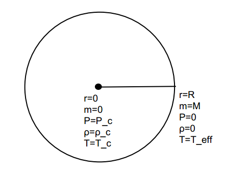
We need to be a bit more careful here about saying what $d-$ scales as what. $dT$ is, properly speaking, the change in temperature between $T_c$ and $T_{eff}$, or $T_c-T_{eff}$. However, since $T_c$ is in the neighborhood of a million Kelvin, and $T_{eff}$ is closer to six thousand, we can say that $dT$ goes as $T_c$ (and $T^3dT$ goes as $T_c^4$). Likewise, $dR$ is $R-R_0$, or $R-0$. Thus, the scaling relationship we end up with is\[T_c^4 \sim \frac{\kappa LM}{R^4}\]The last, and least exciting, scaling relationship comes from $dM = 4 \pi R^2 \rho(r) dr$. We know that $dM$ goes as $M$ and $dr$ goes as $R$, so when we plug in $M/R^3$ for $\rho(r)$, we get\[M\sim \frac{MR^3}{R^3}\sim M\]Not super enlightening, but it does make sense!

This is all we need to go on to start figuring out the scaling relationships we're really interested in. The $T_c$ versus $T_{eff}$ distinction is important when doing the initial derivation, but it turns out that the two scale equivalently, so we'll just use a generalized $T$ from here on out ($T_{eff}$ is ultimately going to matter more anyway). The first relation is mass-radius. We know that $P=\frac{\rho}{\bar{m}}k_BT \sim \frac{M}{R^3}T$, and that $P\sim \frac{M^2}{R^4}$. Substituting for $P$ then gives us $M\sim RT$ or, assuming a constant temperature, $M\sim R$. In other words, mass and radius scale linearly with one another. This will be extremely useful to know very soon.

We'll know look at the mass-luminosity scaling for very massive stars, where $\kappa$ can be assumed constant (meaning that the opacity of the star does not depend on temperature). Based on the scaling relationship we derived from $dT/dr$, this immediately tells us that $T^4\sim LM/R^4$. Now, using the fact that mass and radius scale linearly, we can substitute $M$ for $R$, then solve for $L$. This gives us \[L \sim T^4 M^3\] Or assuming constant $T$, $L\sim M^3$.

For low-mass stars, $\kappa$ gets a little more complicated, following what is known as the Kramer's Law opacity: $\kappa \sim \rho T^{-3.5}$. However, our methodology will be the same, starting with the statement that \[T\sim \frac{\rho T^{-3.5} LM}{R^4}\] Plugging in $M/R^3$ for $\rho$ and substituting $M$ for $R$, this simplifies to $T\sim M^2R^3T^{7.5}$. The reason we left three powers of $R$ in there is because we know, from our scaling relation $M\sim RT$, that $R\sim M/T$. Thus, we can plug this in for $R$ to get our powers of $T$ right (which is nice, though we'll end up considering them as constants anyway). This lets us boil things down to \[L\sim M^5T^{4.5}\sim M^5\]If we assume constant temperature.

Finally, we want to derive the relation between $T_{eff}$ and $L$--this is what lies at the heart of the H-R diagram. Since $L$ = $FR^2$ (luminosity equals flux times area), and that $F=\sigma T^4 \sim T^4$, we know that \[L\sim R^2T^4\sim M^2T^4\] For high-mass stars, we've figured out that $L\sim M^3$, so we'll plug in $L^{1/3}$ for $M$ in this case. This gives us $L\sim L^{2/3}T^4$. Getting all of the powers of $L$ on one side, we have the $L-T$ relationship for high-mass stars as \[L\sim T^{12}\]Pretty steep, huh? Let's see how it looks at the other end of the H-R diagram. For low-mass stars, we found that $L\sim M^5$, so we'll plug in $L^{1/5}$ for $M$. This gives us $L\sim L^{2/5}T^4$. Repeating the process we used for high-mass stars, we get an $L-T$ relation for low-mass stars as \[L\sim M^{20/3}\]Not quite as steep, but still pretty extreme. Since it's clear that the behavior of high- and low-mass stars is somewhat different, it's worth considering an intermediate model, which we'll represent as $L\sim M^4$. The $L-T$ relationship for these stars, derived in the same way, is $L\sim T^8$.

The H-R diagram, in case you forgot (source).

How can this be right when the H-R diagram looks so neatly linear, with the main sequence at such a pretty 45-degree angle? The answer is actually not all that exciting--it's just a question of scaling. Like most plots in astronomy, the H-R diagram is represented on a log-log scale, and while the horizontal axis only spans a few orders of magnitude, the vertical axis covers ten! Looking at the math behind the diagram is a helpful reminder that the best way to represent something visually isn't necessarily the least misleading!

The Taxonomy of Stars

Presented for your consideration: The Hertzsprung-Russell (or H-R, for lazier folks like myself) diagram.

Astute readers will note that this is not the first time this diagram has made an appearance on this blog (source).

This diagram is born of scaling relationships whose derivation I will discuss separately, but the conceptual basis for the H-R diagram isn't too hard to get your head around even without seeing the mathematical justification for it. As you can see, the horizontal axis of the diagram above is surface temperature (actually log$_{10}$ surface temperature), while the vertical axis is luminosity (again, really log$_{10}$ luminosity). These two quantities are, as it turns out, related by a power law--as are mass and luminosity. When astronomers began observing stars, it turned out that they began to fall into pretty specific groups on this diagram, as evidenced by the large empty areas. 

Perhaps the most important feature is the dense line running from the top left to the bottom right, which is known as the main sequence. This is where essentially all stars spend most of their lives, from the start of nuclear fusion up until they begin to die out. Stars which are born larger are brighter, bluer, and hotter (as well as shorter-lived), and as such are in the upper left of the diagram. Dimmer, redder stars are cooler (and longer-lived), and can be found in the bottom right of the diagram. However, a scale of temperatures and luminosities exists between the extremes of the Pistol Star and of Proxima Centauri. Along this scale are the spectral classes of main sequence stars: O, B, A, F, G, K, and M (as well as a few less well-defined and more recently added others). The Sun, for instance, is a rather bright G-type star.

However, stars are not on the main sequence for their entire lives. As stars begin to die, they puff up into giants (or supergiants--or hypergiants!) and do some pretty crazy stuff. In the process, they go careening off the main sequence to the right into the land of giants, where stars like Betelgeuse and Arcturus can be found. Many of the brightest stars in our sky aren't actually main sequence stars, simply because giants are so incredibly massive and luminous.

The star at the center of this cluster--located in the Large Magellanic Cloud--is R136A1, the most massive and most luminous star known (at nearly nine million times the luminosity of the Sun). R136A1 is a Wolf-Rayet star, a type of giant star which is in the process of shedding huge amounts of mass via stellar wind (source).

Once a star has evolved into a giant, it rapidly approaches the end of its life. If the star is big enough (around 10 solar masses) it will collapse in on itself and rebound in a supernova, leaving behind a black hole or neutron star. However, smaller stars--like our Sun--will simply shed their outer layers, leaving behind an incredibly dense core in the form of a white dwarf. What is left behind is a white dwarf, which ends up in the cloud at the bottom of the H-R diagram. These objects are not, strictly speaking, stars, in the sense that they are not experiencing any nuclear fusion. However, white dwarfs are extremely hot when they first form. They do slowly cool, and as a result it is theorized that "black dwarfs"--ancient white dwarfs emitting no heat or light--could exist. However, it is estimated that it would take longer than the current age of the universe for a white dwarf to shed all of its energy, so none yet exist (or at least, they shouldn't!).

Sirius A and B, resolved by Hubble. Sirius A is a bright, nearby A type star (in fact, the brightest star in our sky), while Sirius B is a white dwarf (source).

It seems somewhat incredible that stars should fall so neatly into these categories (and, given that we're still tweaking and adding to the categories, it's clear that it's not that neat), but as we'll soon see when we look at the math behind it, it really does work. Plus, it stands up pretty well to empirical data:

Individual Milky Way stars with H-R regions overplotted (source).

Drunk, Stumbling Photons

Consider a photon that has just been created via a nuclear reaction between two protons in the center of the Sun. The photon now starts a long and arduous journey to the Earth to be enjoyed by Ay16 students studying on a calm Spring day.

a) The photon does not freely travel to the surface of the Sun. Instead it random walks, one collision at a time. Each step of the random walk traverses an average distance $l$, also known as the mean free path. On average, how many steps does the photon take to travel a distance $\Delta r$?

Key to understanding this question is recognizing that photons produced in the Sun do not follow a straight line straight from their source (in this case, nuclear fusion of Hydrogen atoms in the Sun's core) to Earth. Rather, they follow a random walk (alternatively known as a "drunkard's walk"), ricocheting from one proton, electron, or other photon into another in the dense interior of the Sun. Only when they reach the Sun's surface are they free to travel in a straight line.

The random walk of a photon to the Sun's surface (source).

The distance the photon travels during each step of this random walk we have defined as $l$. We'll next define $\vec{D}$ as a sum of vectors $\vec{r}_i$ with magnitude $l$. Since the direction of each vector $\vec{r}_i$ is random, however, then $\vec{D} = \sum \vec{r}_i$ is zero--if if every time you take a step, it's in a random direction, you're ultimately not going to end up very far from where you started. However, you will at times get very far away from your starting point before randomly making your way back, and this is key to understanding photons escaping the Sun. Since the Sun is not infinite, a photon must only make it as far as $R_\odot$ from its source. Once it is at the edge of the Sun, the random walk is over and it is free to propagate into space. Thus, we can remove the directional dependence of $\vec{D}$ by defining $\Delta r$ as $(\vec{D}^2)^{1/2}$. 

Let's begin by solving for $\vec{D}^2$, remembering that it is originally defined as a sum of vectors, from 0 to $N$ (where $N$ is the number of steps it takes to go $\Delta r$ distance--in other words, what we're looking for). Note that, since these are vectors we're dealing with, the multiplication we're doing is actually a dot product. \[(\sum_{i=1}^N \vec{r}_i)^2 = \sum_{i=1}^N |\vec{r}_i||\vec{r}_i| cos(0) + \sum_{i,j}|\vec{r}_i||\vec{r}_j|cos(\theta)\] $\theta$ is the angle between vectors $\vec{r}_i$ and $\vec{r}_j$, which, since the directions of  $\vec{r}_i$ and $\vec{r}_j$ are random, is an expectation value for an "average" direction. Mathematically, we can define it as \[\frac{1}{2\pi}\int_0^{2\pi} cos(\theta)d\theta = 0\] Thus, the second term in our squared summation is simply zero. As for the first term, since $|\vec{r}_i|$ is by definition $l$, we have \[\sum_{i=1}^N |\vec{r}_i||\vec{r}_i| cos(0) = \sum_{i=1}^N l^2 = Nl^2\] Remembering that this is equal to $\vec{D}^2$, we can next take the square root of $Nl^2$ and set it equal to $\Delta r$. Finally, we can solve for $N$, giving us \[N = (\frac{\Delta r}{l})^2\]

b) What is the photon's average velocity over this distance? Call this $v_{diff}$, the diffusion velocity.

Having wrapped our heads around the fact that a photon must actually travel $Nl$ distance in order to get $\Delta r$ away from its source, figuring out $v_{diff}$ is just a distance equals rate times time problem. We'll start by actually calculating $t_{diff}$, the diffusion time, since we know that the photons are actually moving at rate $c$--the speed of light--just not aways in the right direction. Thus, $Nl = c \times v_{diff}$, So $t_{diff} = \frac{Nl}{c}$. Plugging this all back into the distance-rate-time setup, we can now say that \[\Delta r = v_{diff} \times t_{diff} = \frac{v_{diff} Nl}{c}\] Solving for $v_{diff}$ gives us \[v_{diff} = \frac{\Delta r c}{Nl} = \frac{\Delta r c}{\frac{(\Delta r)^2}{l^2}l = \frac{cl}{\Delta r}\]

c) The `mean free path' $l$ is the characteristic (i.e. average) distance between collisions. Consider a photon moving through a cloud of electrons with a number density $n$. Each electron presents an effective cross-section $\sigma$ . How are these parameters related?

Electrons are pretty small, but they still do have a physical size. This is represented here by the quantity $\sigma$, which can be thought of as the "diameter" of a particle. Larger particles--such as protons and neutrons--have larger cross-sections, and are thus photons are more likely to hit them and scatter. Likewise, if particles are more dense, photons are similarly more likely to hit them and scatter.

Density and cross-section $\sigma$ of electrons in a volume of length $dx$ (source).

Establishing a relation between $l$, $n$, and $\sigma$ really is this simple. Since larger values of both $\sigma$ and $\n$ will yield smaller values of $l$--particles scattering more often will travel less far in between each instance of scattering--we can establish the relation $l = \frac{1}{\sigma n}$. A quick unit check shows that this works out dimensionally as well.

d) The mean free path length $l$ can also be related to the mass density of absorbers $\rho$ and the absorption coefficient $\kappa$ (cross-sectional area of absorbers per unit mass). How is $\kappa$ related to $\sigma$? Express $v_{diff}$ in terms of $\kappa$ and $\rho$ using dimensional analysis.

Once again, increasing both mass density and absorption will decrease $l$, so we can state that $l = \frac{1}{\kappa \rho}$ (and again, the units reassuringly check out). We can then just plug these in for $l$ in our equation for $v_{diff}$, which tells us that \[v_{diff} = \frac{c}{\kappa \rho \Delta r}\]

e) What is the diffusion timescale for a photon moving from the center of the sun to the surface? The cross section for electron scattering is $\sigma_T = 7 \times 10^{-25}$ cm$^2$ and you can assume pure atomic hydrogen for the Sun's interior. 

We computed $t_{diff}$ way back in part b) as $\frac{Nl}{c} = \frac{\Delta r^2}{cl}$. We can now apply this here, using $R_\odot$ as $\Delta r$ and $\frac{1}{\sigma n}$ for $l$. The first step is to find $n$, which we can do by dividing the mass density of the Sun, $\rho_\odot = 1.5$ g cm$^{-3}$ by the mass of a hydrogen atom, $\bar{m} = 2 \times 10^{-24}$. All of this can then be plugged into our equation for $t_{diff}$. \[t_{diff} = \frac{R_\odot ^2 (\frac{\rho_\odot}{\bar{m}})\sigma_T}{c}=\frac{(7\times10^{10})^2\times1.5\times7\times10^{-25}}{2\times10^{-24}\times3\times10^{10}}\] This all comes out to about $10^{11}$ seconds--or more usefully expressed, 10,000 years. This means that, while it may take only eight minutes for a photon to travel one AU from the surface of the Sun to Earth, it took that photon billions of times as long just to travel less than .5% of the distance. Interestingly, it also means that if the Sun were to "go out" today, ceasing all production of energy in its core, we wouldn't find out until countless generations from now.

Everything Falling Together (More on Molecular Clouds)

The time scale of star formation and stability: The time for a self-gravitating cloud to collapse is often estimated by the "free-fall timescale," or the time it would take a cloud to collapse to a point in the absence of any resistance. We'll derive this timescale and use it to re-derive the Jean's Length.

a) Consider a test particle in an $e=1$ "orbit" around a point mass and use Kepler's Third Law to derive a general equation for the free-fall time. Recall that $e=0$ describes a circular orbit, and make sure you draw what an $e=1$ orbit looks like. Use $m=4\pi r^3 \bar{\rho}$ to frame this expression in terms of a single variable--the average density, $\bar{\rho}$.\[t_{ff} = (\frac{3\pi}{32G\bar{\rho}})^{1/2}\] What assumptions are implicit in the last step?

The key to this problem has more to do with understanding exactly what it's asking than with any real mathematical complexity. What we're trying to do here is approximate the free-fall time of a molecular cloud as a Keplerian orbit, treating the mass of the cloud as a point mass at one of the foci. However, since we're looking at an $e=1$ "orbit"--an orbit with eccentricity of 1--the foci are actually at the ends of the ellipse, and the ellipse is actually a line (technically a special case of an ellipse, the same way a circle is). This way, we can plug everything into Kepler's third law and use $1/2 \times P$ (where $P$ is the period) as $t_{ff}$. For me, it was mist intuitive to imagine the entire cloud as having a radius $r$ but having all of its mass concentrated in the center. The test particle, then, is "orbiting" the center of mass of the cloud with $e=1$, starting at the edge and going directly toward the center. $r$, then, is also double the semi-major axis of the particle's "orbit."

The radial line is both the radius of the cloud and double the semi-major axis of the particle's $e=1$ "orbit." The mass of the cloud, $M$, is concentrated in a point mass at the center.

Plugging all of this into Kepler's third law gives us \[P^2 = \frac{4 \pi^2 a^3}{G\frac{4}{3}\pi r^3 \bar{\rho}}\] We can then plug $2a$ in for $r$ and do some canceling to get \[P^2 = \frac{3 \pi}{8 G \rho}\] Finally, we substitute $(2t_{ff})^2 = 4t_{ff}^2$ for $P^2$ and divide across by the $4$. Taking the square root of both sides gives us \[t_{ff} = (\frac{3\pi}{32G\bar{\rho}})^{1/2}\]The largest assumption that we are making here is, of course, that Kepler's third law holds up in the extreme case of an object with no angular momentum simply falling into another object. However, just as a circle (one extreme case of an ellipse) holds up, it seems logical that a line (the opposite extreme case) would as well. Likewise, Kepler's third law holds for an object on a massively elliptical orbit that comes within spitting distance of the central mass at one end of its orbit and is incredibly far away at the other end--this type of orbit is characteristic of Oort Cloud comets which are hundreds of AU away at aphelion but get close enough to the Sun at perihelion to start vaporizing (this is where the tails of comets come from). Stretching that orbit out a bit further into a line should work (even if it means we're firing a hypothetical comet into the Sun).

b) If the free-fall timescale of a cloud is significantly less than a "dynamical timescale," or the time it takes a pressure wave (sound wave with speed $c_s$) to traverse the cloud, the cloud will be unstable to gravitational collapse. Use dimensional analysis to derive the relationship between the sound speed $c_s$, the cloud's pressure $P$, and the mean density $\bar{\rho}$. Then derive the dynamical timescale $t_d$, the time it takes a pressure wave to cross the cloud of radius $R$.

Right off the bat we know we're relating a velocity to a pressure and a density. The units of velocity are, of course, m s$^{-1}$. Density is just mass per volume, or g v$^{-3}$. Pressure, meanwhile, is a force per unit area--g cm$^{-1}$ s$^{-2}$. The only step required to relate these quantities is to square $c_s$, multiply it by $\bar{\rho}$, and set them both equal to $P$, giving us\[P = c_s^2 \bar{\rho}\]In order to find the dynamical time, we can just think of it as a distance equals rate times time problem--$c_s \times t_d = 2R$, since the dynamical time is defined as the time required for a wave moving at speed $c_s$ to cross a cloud of diameter $2R$. Solving for $t_d$ is a simple matter of dividing both sides by $c_s$, then plugging in $(\frac{P}{\bar{\rho}})^{1/2}$ for $c_s$.\[t_d = \frac{2R}{(\frac{P}{\bar{\rho}})^{1/2}} = \frac{2R\bar{\rho}^{1/2}}{P^{1/2}}\]

It's tough to find any relevant images that aren't in graph form, so here's another pretty molecular cloud. This one is Messier 17, also known as the Swan (or Omega) Nebula (source).

c) Equate the free fall time to the sound crossing time and solve for the maximum $R$. This
maximum is Jeans Length $\lambda_J$.

Just some straightforward algebra here. We start with \[t_d=\frac{2R}{(\frac{P}{\bar{\rho}})^{1/2}} = \frac{2R\bar{\rho}^{1/2}}{P^{1/2}} = (\frac{3\pi}{32G\bar{\rho}})^{1/2} = t_{ff}\]Multiply over the $(\frac{P}{\bar{\rho}})^{1/2}$ and divide both sides by 2 and we've solved for R, giving us \[R = \lambda_J = (\frac{3 \pi P}{128 G \bar{\rho}^2})^{1/2}\] What this means is outlined in the setup for part b), but to reiterate--when the cloud gets below this length, the free-fall time will be less than the time it takes for a pressure wave to cross the cloud. As a result, pressure will no longer be able to counteract the force of gravity, and the cloud will collapse.

d) You have just performed an order of magnitude derivation of the "Jeans Length." A more careful derivation yields the following definition:\[R_J=(\frac{\pi c_s^2}{G\bar{\rho}})^{1/2}\] where $c_s$ is the isothermal sound speed. What are we assuming in using the isothermal sound speed? Discuss amongst your group the significance of this characteristic length within the cloud.

The significance of $\lambda_J$ is outlined above, but the assumptions made in using the isothermal sound speed are worth examining. The most significant assumption is that the cloud itself really is isothermal--the same temperature everywhere. This means that it is diffuse enough that any photons emitted from inside of it can make it out without getting scattered back in by interactions with gas particles. When the cloud gets much more compact, this ceases to be the case, the mechanics of collapse become quite a bit more complicated. However, for a cloud of a few thousand solar masses that may be dozens of light-years from side to side, it is reasonable to assume it is isothermal.

e) For simplicity, consider a spherical cloud collapsing isothermally (constant temperature, $T$) with initial radius $R_0 = R_J$. Once the cloud radius reaches $R=0.5 R_0$, by what fractional amount has $R_J$ changed? What might this mean in terms of the number of stars formed within a collapsing molecular cloud? (This is the concept of fragmentation.)

What we're interested in here is how $R_J$ changes compared to $R$, so we should start by solving for $R_J$ in terms of only $R$ and constants. We're pretty close to this already, with the equation we're given in part d). However, this is given in terms of density, which will change as the radius of the cloud shrinks. Instead, let's plug in $\frac{M}{4/3\pi R^3}$ for density, cancel the $\pi/3$, and lump all of our $R$ terms together. This gives us\[R_J = R^{3/2}\sqrt{\frac{4\pi c_s^2}{GM}}\] Everything in the square root will stay constant, so let's just call it $x$--it doesn't really tell us how $R_J$ changes with $R$. We end up with $R_J = xR^{3/2}$.

Let's now think about the relationship between $R_{J,0}$, the initial Jeans length with $R = R_0$, and $R_{J,1}$, the Jeans length when $R = 1/2R_0$. \[R_{J,1} = x \times (1/2R_0)^{3/2}=\frac{x}{2\sqrt{2}}R_0^{3/2} = \frac{1}{2\sqrt{2}}R_{J,0}\] So even though the radius is now $1/2$ times its original size, the Jeans length is $\frac{1}{2\sqrt{2}}$ times its original size! This is key, because it means that when a cloud begins to collapse from its Jeans length, there will come a point where he ratio of the Jeans length to the radius is small enough that multiple areas within the cloud will begin to collapse independently. The process will then repeat in each of those "sub-clouds," until--rather than forming into one colossal star--the cloud has fragmented into an enormous number of smaller stars.

Fragmentation of a molecular cloud into newly-formed protostars (source).

Once again, credit and thanks for collaboration on this problem go out to my partners in crime Scott Zhuge and Anne Madoff, without whom I would still be bumbling around trying to figure out the first step.